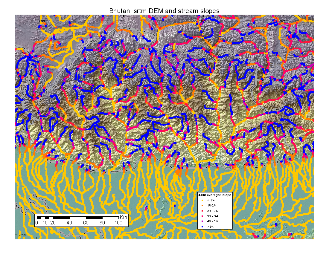
Calculating stream slopes from world DEMs
HydroSHEDS
Worldwide DEMs such as the SRTM DEM, especially the publicly available
3" (~90m) version, leave one struggling the define channels,
much less calculate slope.
We have leaned heavily on the
HydroSHEDS version of the SRTM DEM. Longitudinal
profiles of rivers were created by tracing from cell center to cell center.
These profiles never (in the conditioned DEM) run uphill, and their geographic
coordinates follow the actual rivers as well as human experts could determine.
However, slopes cannot be trusted, if only because they are often stairstepped,
with apparent flat spots and bogus waterfalls. Even a perfect DEM will
generate problems in all but the steepest rivers when elevations are rounded
to the nearest meter.
Once a profile graph is extracted from the GIS, there are myriad ways to smooth
it. We adopted the strategy of extending our smoothing window to the next
highest and lowest points, and imposing the additional constraint of looking
a minimum distance (1, 2 or 4 km) upstream and downstream. The results can be
seen below.

ASTER Global 1" DEM
Then we decided to extract better elevations from the DEM.
While we were still mulling over techniques of doint this with the SRTM DEM,
the 1" (~30m) Global DEM became available. Maintaining the stream points
from hydrosheds (version 3?) as our offical river course, we
- Converted the points to 1" cells in the space of the Global DEM.
As the GDEM cell centers fall on the edges of Hydrosheds cells, there is a
uniform 0.5" shift, but this does not worry us. In fact it partly
compensates for the 1.5" NE shift of the HydroSHEDS data.
- Calculated the locus of 1" grid cells closest to each streampoint,
clipping to an arbitrary buffer of .05 degrees.
These regions, called Thiessen polygons or Voronoi cells before clipping,
were computing with the eucallocation function in ARC/INFO.
- Found the lowest elevation within each region. (zonalmin)
- Assigned that elevation back to the point.
- For diagnostic purposes, those lowest cells were converted to points and
are displayed below as stars. In the case of ties, more than one point
may be shown.
For the Wang Chhu, the buffer size looks good. Too small a buffer will fail
to catch useful points. Too large a buffer will catch points that are
legitimately lower than the river channel.

| 
|
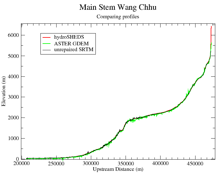
| The Wang Chhu is the major river of Bhutan.
It continues across the India before joining with other rivers,
entering Bangladesh, and flowing toward the Brahmaputra.
|
| Here are three versions of the profile of the
Wang Chhu. The hydroSHEDS profile looks well behaved, though the flat
regions are unlikely to be real. The SRTM DEM is shows some spikiness.
It would have looked better if we had been able to obtain a 3" DEM
generated as the minimum of the 9 component 1" values. The ASTER GDEM is
more spiky, and it shows some low spots that we would like to take a look at.
|
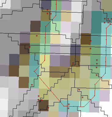
| 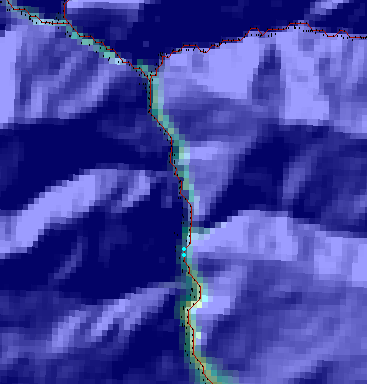 |
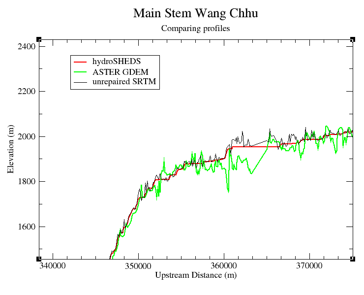
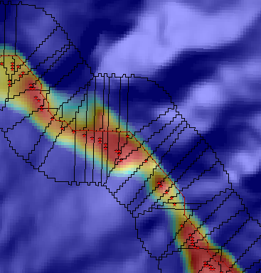
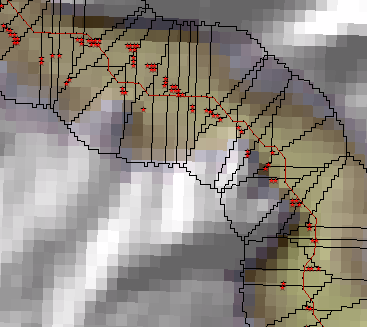
| Above is the SRTM image of an area in the second box of the context map.
The graph on the left is a detail of the full river profile.
This area concerns us. If the GDEM contains
bogus pits, our data filtering becomes much more difficult.
The image on the right shows the 3" hydroSHEDS DEM, the profile created
from it, and red points selected where the GDEM elevations were selected.
The two big blue points are the troublesome pit on the graph.
|
|
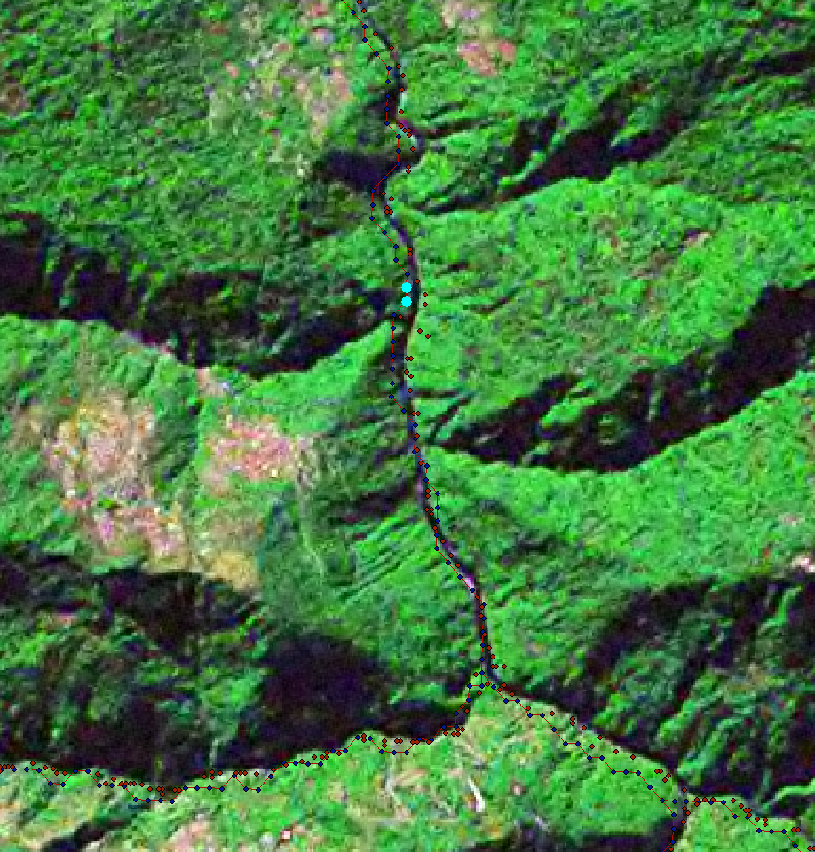
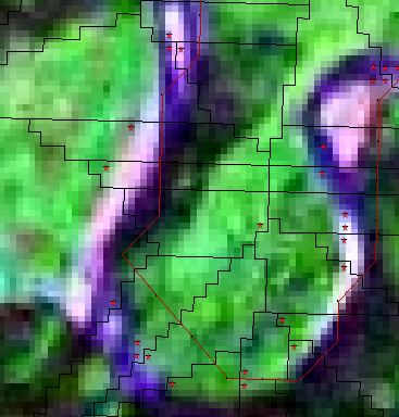
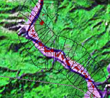
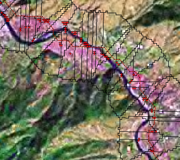
| This is a [15m lossy] Landsat image of the same area.
It is flipped upside down for those of us who cannot interpret
aerial/satellite photos illuminated from the bottom.
|
|
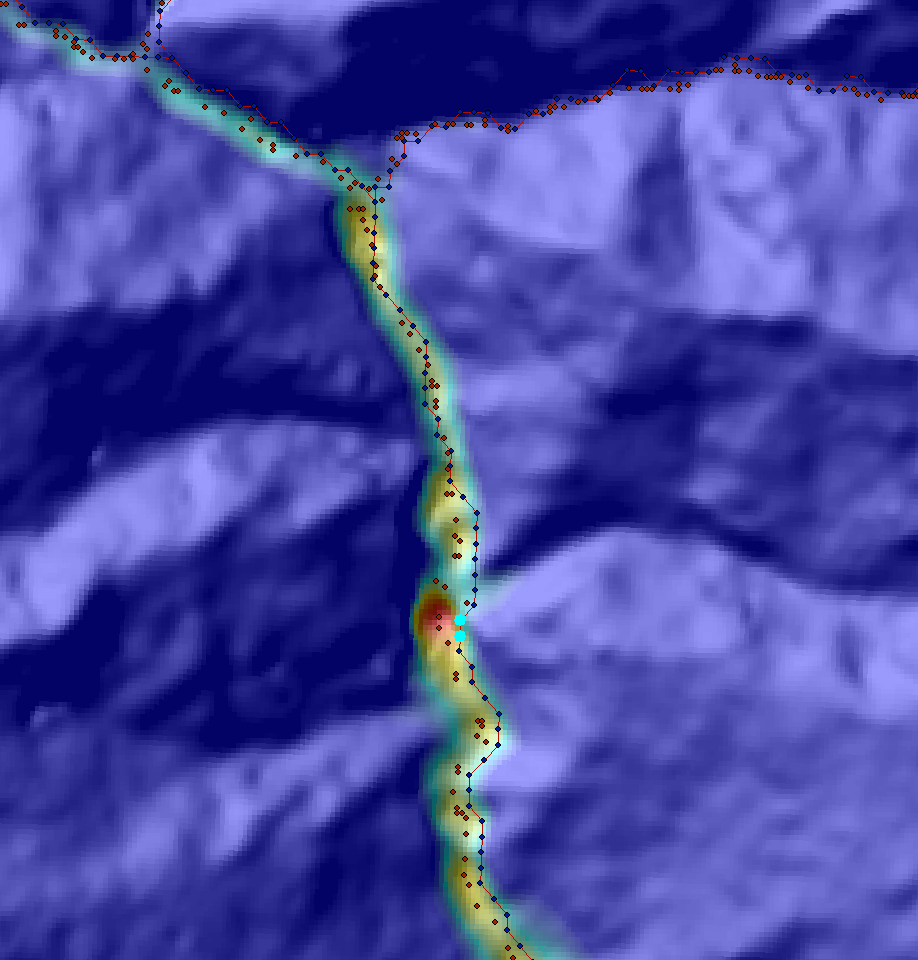
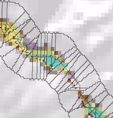
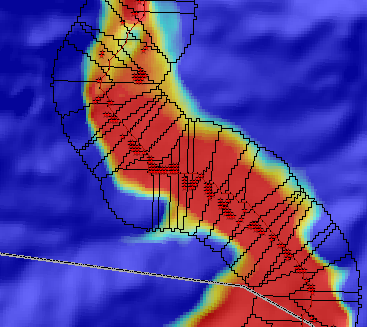
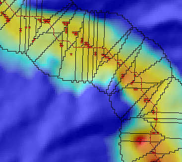
| This is the 1" Global DEM with a special color stretch. The dip
in our river profile is clearly visible as a feature of the river channel,
comprising many data points and centered on the channel. This leads us
to conclude that these are legitimate elevations, and that apparently
higher areas downstream are artifacts of tree cover.
The two pixels have 9 and 10 components values (The minimum value from 9 ASTER
scenes was used.). This is typical for the area, though it seems that
high points on the profile have lower data quality. We will look at
this statistically later.
|
| 
| 
|
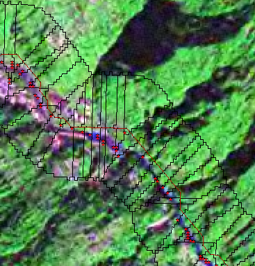
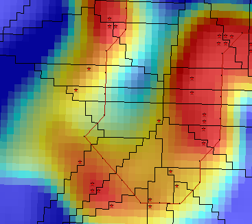
| Here is one artifact of my clever method.
Profile points has a small
search area on the inside of curves. If the actual channel lies to the inside
of the curve, that particular HydroSHEDS point is inhibited from searching
the channel for a data point. The result is a spike in the profile.
This is not a big problem, as we expect upward spikes and remove them.
|
| 
| 
|
| Here is a similar artifact. Because of a poor match between
the profile and the actual channel, a profile point has serched across an
oxbow to find a data point. Such an error could result in a downward spike,
but here it merely produces an upward spike.
|
| 
| 
|
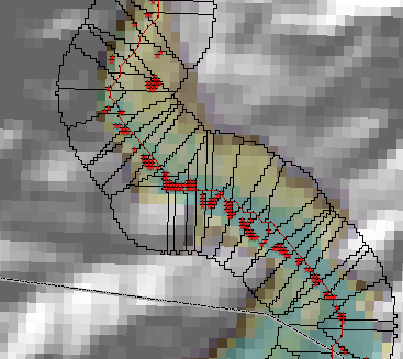
| Here we see our methodology start to fall apart
as the Wang Chhu becomes
a braided river near the Indian border. The river has moved considerably
between the Landsat (~2000), SRTM (Feb, 2000?), and multiple ASTER passes.
|
| 
| 
|
| This is the first place where I suspect that a floodplain
is lower than the surface of the river. This is way upriver at about
2000 meters.
|
For the most part, the GDEM points define the channel better than HydroSHEDS,
but there is some unacceptable noise in their path. Would it be possible to
automate a redefining of the channel course? Would it be worth while to build
a GIS team in Bhutan to refine the data sets?
Don't forget tie scores. And what if we constructed perpendicular bisectors at each and searched for an alternate lowest point? Not so good, I suppose.
Now we have revisit our smoothing algorithm. For now we will assume that
all bumps are artifacts and that no low points will be discarded. As our
data is in integer meters, we cannot (except where points are discarded)
represent non-zero slopes less than one meter over thirty meters.
This is unacceptable even in Bhutan.
We have run this procedure on most of the Brahmaputra basin, and are
starting to evaluate the results.
GDEM2
Version 2 of the ASTER Global DEM looks much better. We are looking forward
to testing it with our existing algorithms.