We are looking at ways of defining the basin and flow directions.

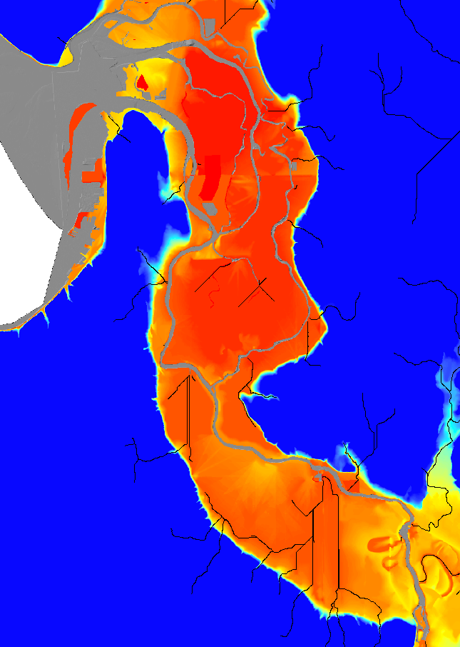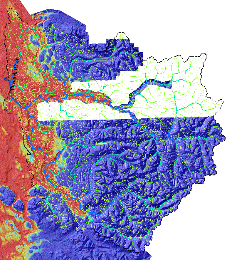
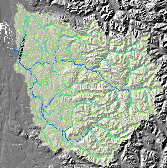
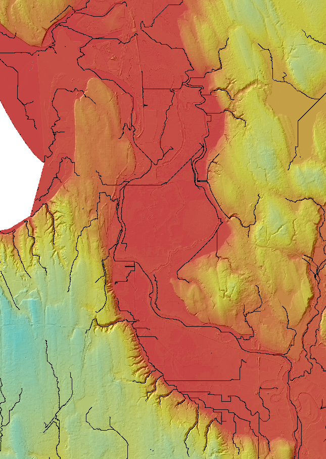
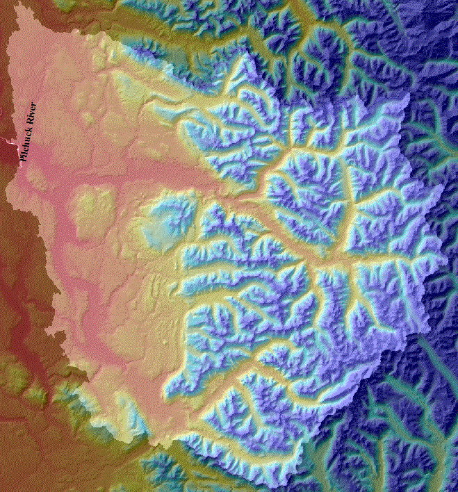
Here are streams, calculated from the 10-meter DEM (derived from USGS 1:24000 topo sheets) laid over the DEM. Uplands are blue. Water shown in gray, including much of the river, is no-data and is not modeled.	Here are streams calculated from the LiDAR DEM, laid over the LiDAR DEM. Of course, they require pruning in the Sound.
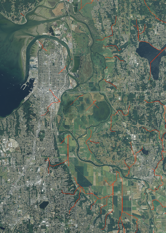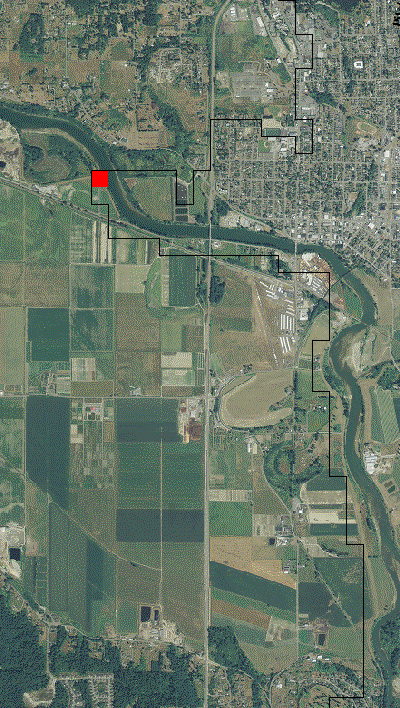
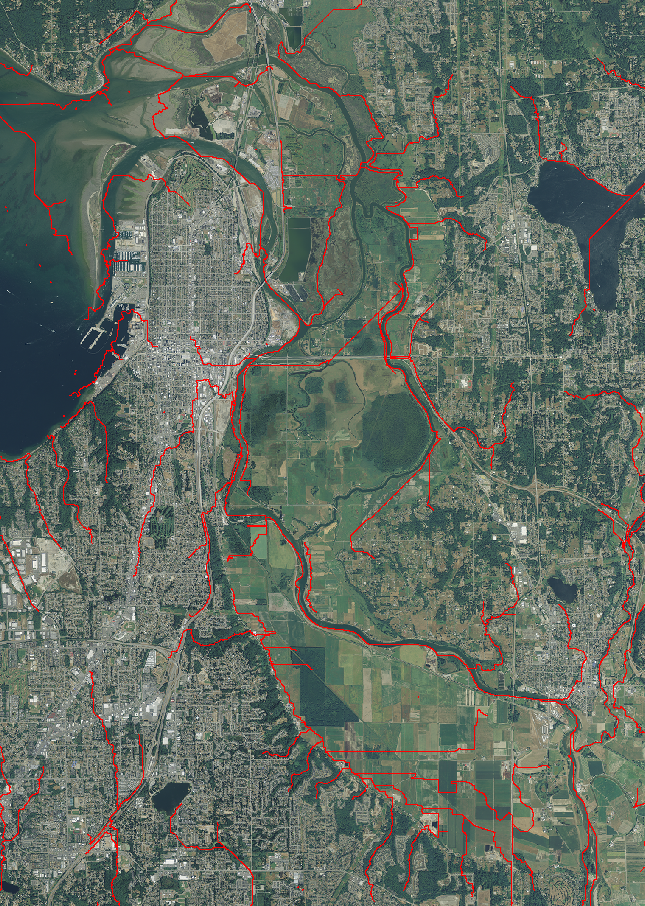
Here are the same 10-meter streams laid over the 2009 NAIP orthophoto	And the LiDAR-derived streams laid over the photo.
	The flow directions shown above can be altered to suit the modelers, and the basin outlet can be moved up and down stream. Parts of the estuary can be modeled as separate small basins.
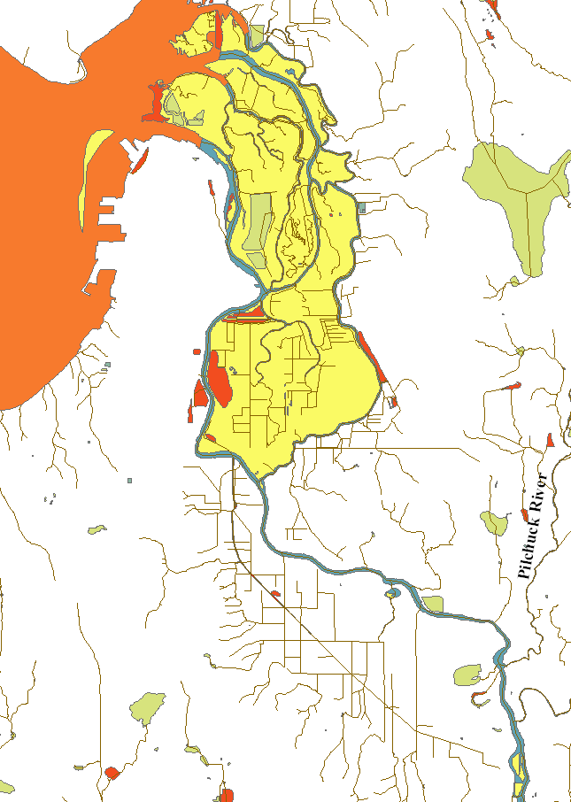
This is the DNR water body (and island) polygon and line shapdefile

		We have decided to model a single basin with a pour point west of Route 9. This yields a watershed that includes the Pilchuck River, and which extends further north than the previous DHSVM models.
		First the 6-foot LiDAR DEM, which covers most of the basin, was reprojected to UTM NAD27 at two-meter resolution. This data was aggregated to ten-meter resolution by Filled, calculated flow direstion and accumulation at two meters Aggregated maximum flow accumulation to ten meter, and took the natural log Aggregated minimum and mean elevation to ten meters. Created a ten-meter DEM based on a weighted average of the aggregate minimum and mean elevations, assigning the minimum aggreate elevation where ln(accumulation) was highest and the mean aggregate elevation where ln(accumulation) was low. This created a ten-meter elevtion grid that tended to respect flow directions observed on the detailed DEM.
		This DEM was merged with the USGS ten-meter DEM to fill in places where LiDAR data was absent. Flow directions and accumulation were created from this ten-meter DEM. This information was carefully examined with WRIA boundaries, orthophotos, DNR streamlines, and LiDAR data, and the flowdirectin grid was manually corrected until we were satisfied with ten-meter flowlines and boundaries.
		The ten-meter flowdirection grid was aggregated to 150 meters by examining all flows that cross the 150-meter edges and summing the net flows to determination the maximum net flow direction. The results were examined, and minor corrections were done the create the revised basin shown here.

1999 Snohomish work