| Name | Last modified | Size | Description | |
|---|---|---|---|---|
| Parent Directory | - | |||
| z.tfw | 2018-12-12 15:59 | 88 | ||
| READ_ME.txt | 2018-10-05 15:35 | 355 | ||
| z.aux.xml | 2018-12-12 15:59 | 2.5K | ||
| z.xml | 2018-12-12 15:59 | 5.8K | ||
| fuzzytest.lyr | 2018-10-05 15:34 | 12K | ||
| transects.png | 2018-12-10 12:44 | 42K | ||
| southslope.png | 2018-12-10 12:30 | 57K | ||
| fig_lidar_smooth.png | 2018-11-29 13:26 | 65K | ||
| lidar.png | 2018-11-16 15:47 | 70K | ||
| fig_lidar.png | 2018-11-28 16:13 | 97K | ||
| fig_mosaic.png | 2018-11-29 14:07 | 377K | ||
| fig_acc_tryptich.png | 2018-12-10 15:45 | 534K | ||
| acc.png | 2018-12-10 14:38 | 583K | ||
| fig_acc_3algo.png | 2018-12-19 16:19 | 622K | ||
| fig_acc_melded.png | 2018-12-11 14:17 | 865K | ||
| april_acc_melded.png | 2019-04-29 13:54 | 9.2M | ||
| hillshade_bumped.tif | 2018-12-11 14:00 | 9.4M | ||
| z.ovr | 2018-12-12 15:59 | 25M | ||
| z.tif | 2018-12-12 15:59 | 86M | ||
| southslopem1acc.tif | 2018-11-16 15:15 | 102M | ||
| testacc.tif | 2018-11-15 15:55 | 102M | ||
| acc_cm.tif | 2018-12-09 14:30 | 109M | ||
| fuzzytest.tif | 2018-10-05 15:32 | 131M | ||
| southfill_1m.tif | 2018-10-05 15:38 | 1.2G | ||
| fuzzysouth.tif | 2018-12-13 15:48 | 1.4G | ||
This is the bare beginning of a web page. It will be filled in with more images, hyperlinks, and discussion.
The primary work directory is e:/dryvalleys on dusty in the puppetlab (JHN376). Some files were saved on the group fileserver at y:/topog/areas/dryvalleys. This page is on the web server w:/areas/dryvalleys
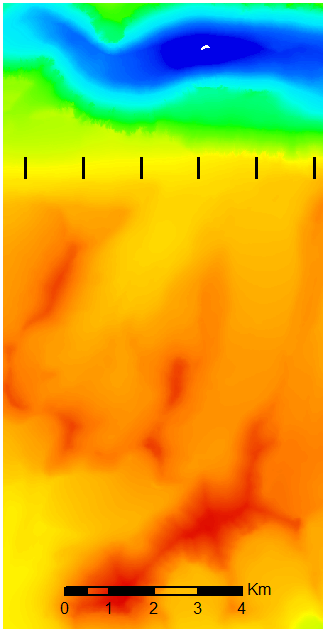 | 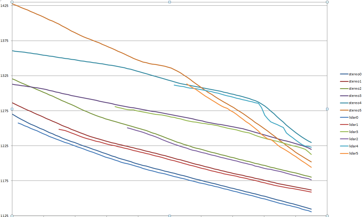 |
| In a 3600-by 7050 window, the lidar DEM was laid over the Satellite DEM, preserving the no-data lake in the lidar DEM. (It was a big mistake to try it without preserving the sink. The results of this mistake are preserved as southslope_nonodata.tif and southslopetoomuchfill.tif.) | Six transects show the difference between the aerial lidar and satellite images where they meet. In happens that all six transects show the aerial images being lower, but and examination of accumulated area will show a few places where the aerial lidar is higher. |
| Flow accumulation methods There are various methods of calculating flows (of water or whatever) across the landscape. The simplest method is to assume that all the water in a cell flows to its lowest neighbor. (Things are slightly more complicated when there are closed depression which are do not drain into noData cells, or when there are flat areas as can occur by chance or when closed depressions are filled by pre-processing the DEM.) This works well for streams (if you don't mind their being one cell wide, and having no braiding or deltas), but works badly for hillsides. ESRI offers an "MDF" flow flow direction option, and can use MFD files to drive the flowdirection function. However, ... | |
| In order to have the minimum size undrained sink at the bottom of the valley, we expanded the noData area. After a few iterations ("more_sinks" and "sinks641" in e:/dryvalleys, we settled on "sinks6417", with all cells below 64.17 meters being redefined as noData. As it turned out, all this effort made little difference. | |
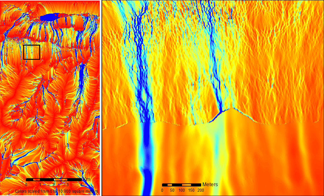
We filled all the sinks in the default ESRI manner, and calculated flowaccumulation with shalstab.py The black box indicates the part of the image which is blown up on the right. The blue fish-shaped area near the top is an area where the shalstab.py algorithm breaks down. It is not important to this analysis, but we are looking into the problem. | |
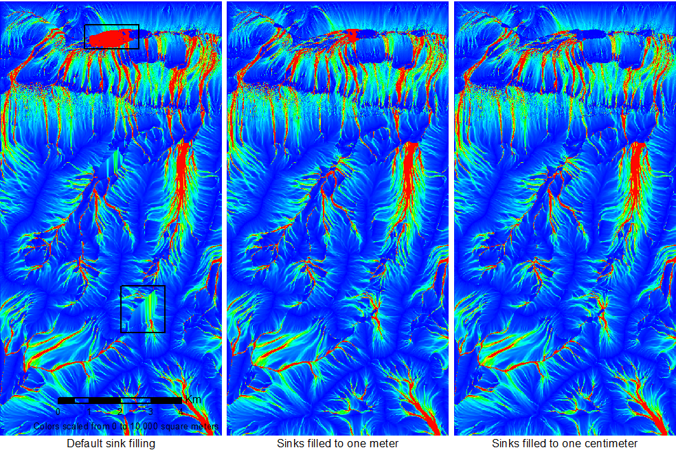 | |
| In the lower box of left-hand figure, we see a region of fuzzy parallel flow lines. This is because sinks have been filled, and that region is represented as flat when flows are calculated. In the second figure, we filled only those sinks less than one meter in depth. Flows in that are represented better, but total flows throughout the landscape are diminished as flows enter sinks and stop. In the third figures, there is even less sink filling. Note the fish-shaped figure in the top box. For reasons we have not determined, this artifact is reduced when there is less sink filling. | |
| |
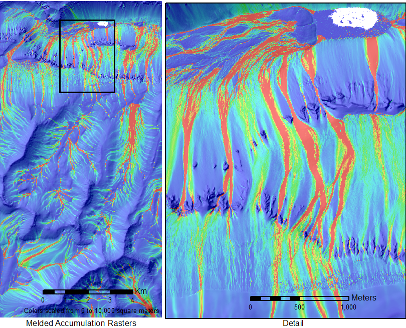
| Our ultimate flow-accumulation product melds the three versions, using the default full-sink-filling version for most of the landscape, but substituting data from the other two models where the first model does not represent the flows well. (The underlying shaded-relief image was made with "resolution bumping", where the DEM was averaged with a smoothed DEM before hillshading. This emphasizes general forms without completely obscuring fine details. | |
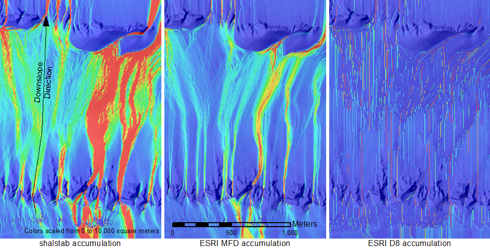 three methods.
A simple example
shows how strange the ESRI algorithm is.