• what the Continental Ice Sheet did to Western Ontario
• how the CDED DEM surpasses the ASTER Global DEM in clarity, at least in the well-surveyed south.
• how resolution bumping improves (though Jay Hart is not persuaded by my example) the readability of shaded relief imagery
• How one-meter resolution DEMs cause stairstepping in shaded relief.
• Adjustments in parameters for hillshading in geographic coordinates for display in equidistant coordinates.

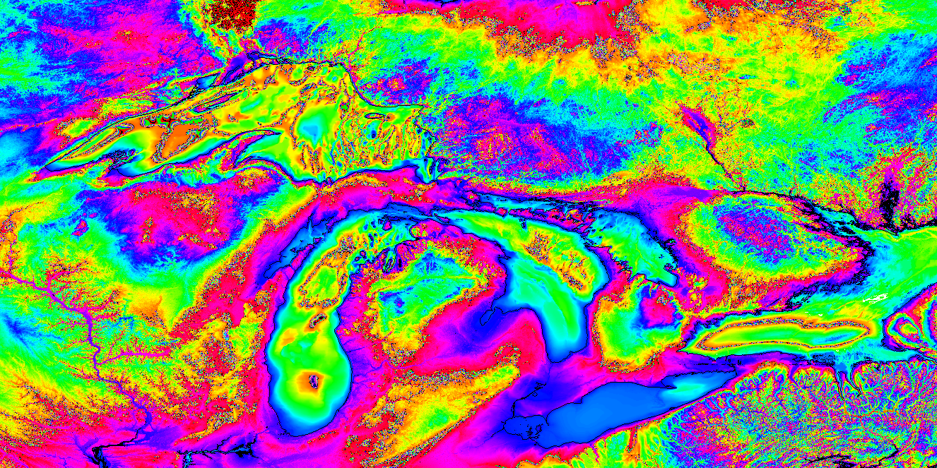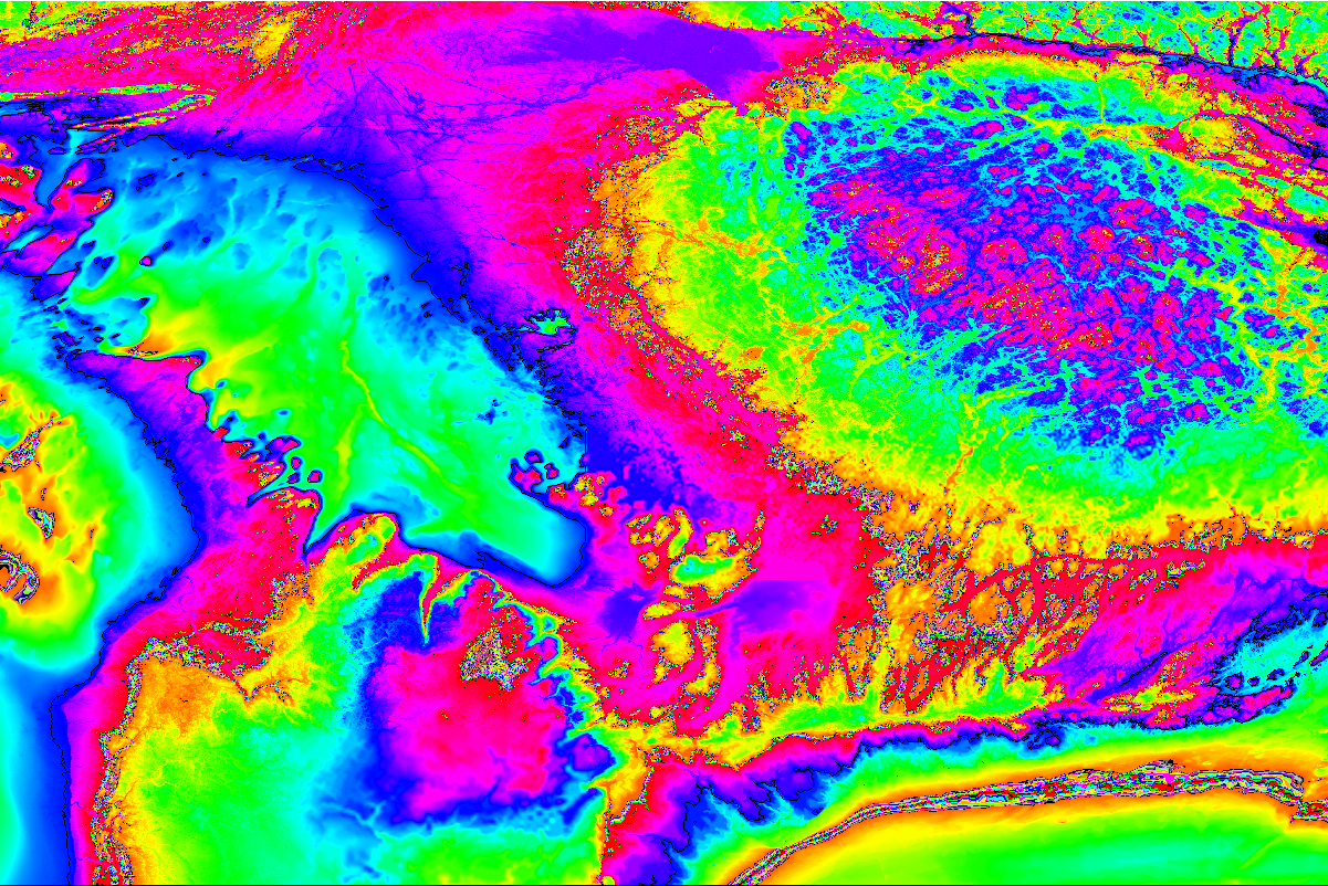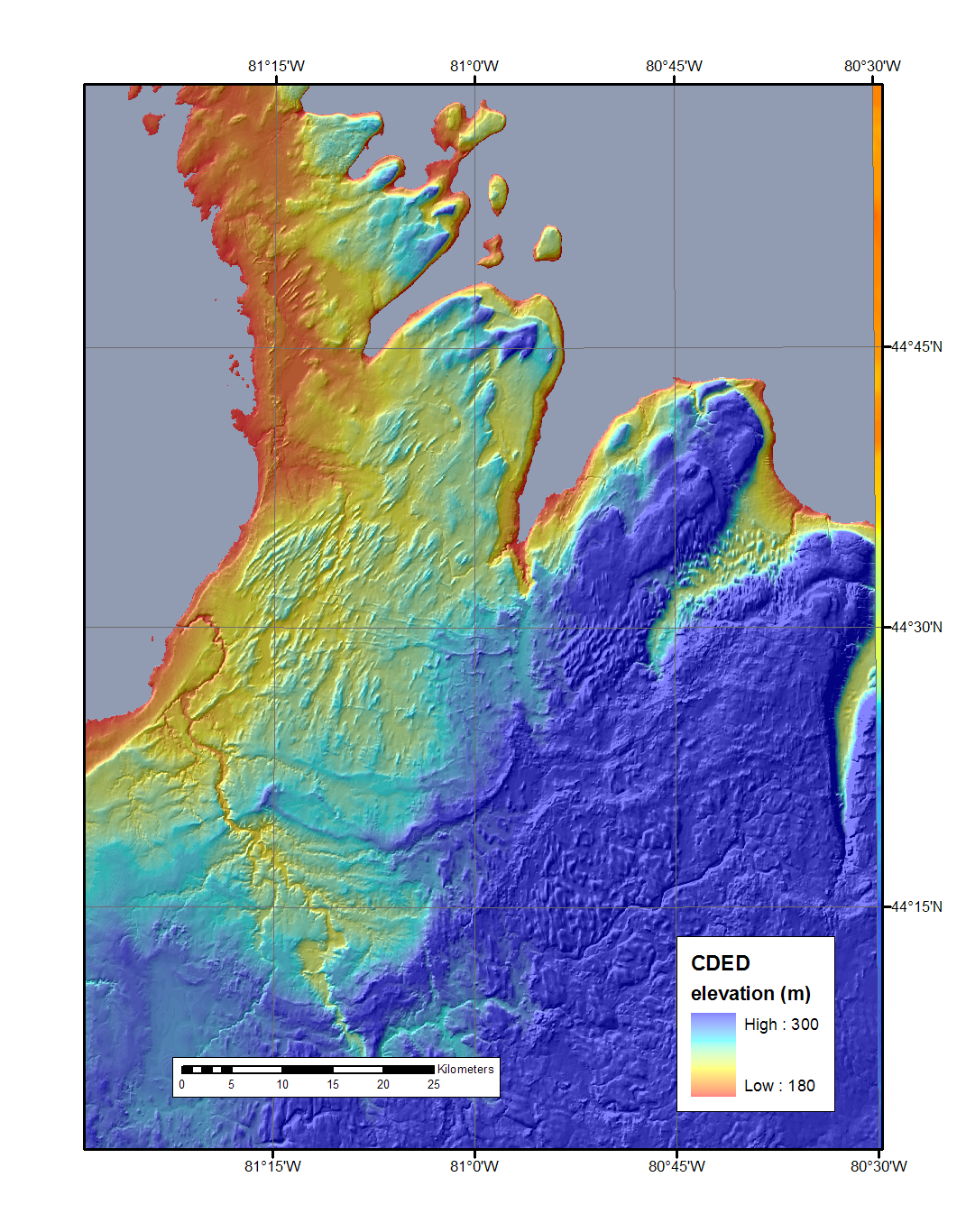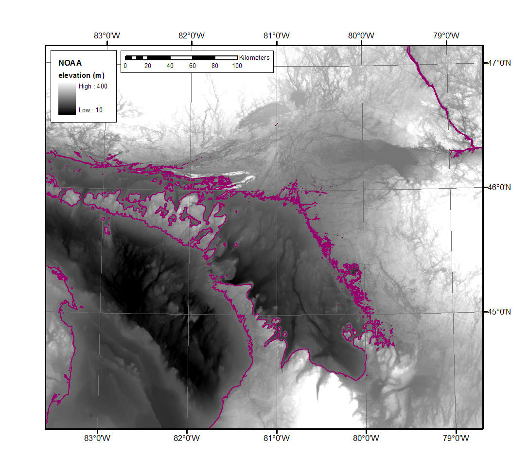
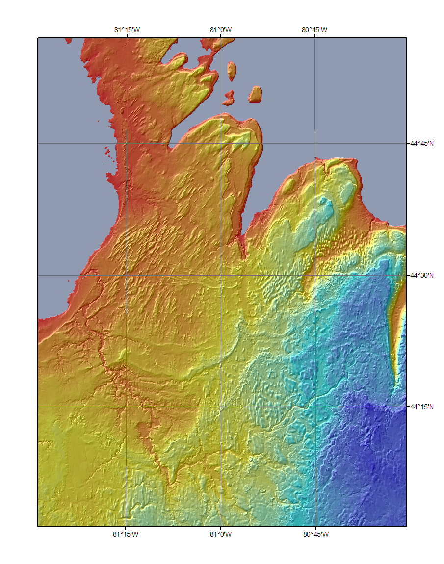
A "shaded relief image" is a mathematical model of how a digital elevation model would look if illuminated from from a given direction. The actual albedo and color of the landscape are ignored. Essentially, a shaded relief image mimics a plaster-of-Paris model illuminated by one distant spotlight. The effects of oblique lighting are modeled. The model could be asked to portray shadows, but that is seldom desirable. It is sometimes useful to mimic actual solar positions, but images are easiest to read when illuminated from the upper left at an elevation of 30-45°. The images seen here are color coding of elevation transparently laid over shaded relief. Here we lit the model from an azimuth of 315°, measuring clockwise from north, i.e. the northwest. This angle is only approximate when we run the model on data in geographic coordinates (degrees of latitude and longitude) as a square degree is not close to a square on the ground unless you are at the equator. The shape of cells is compressed by the cosine of the latitude.

Let's do the math, assuming a spherical earth. It is easiest to work in Cartesian angles, measuring counterclockwise from eastward rather than in bearings (as used by ESRI to calculate shading) measured clockwise from northward. Thus the standard azimuth (sunlight coming from the northwest, i.e. bearing of 315 degrees) is 135 degrees, or 135 / (π×2) radians. In equidistant coordinates, the X and Y components are cosine(azimuth) and sine(azimuth). In geographic coordinates, the X component becomes cosine(azimuth) / cosine(latitude). So a bearing of 315 degres at a latitude of 44.5 degrees would be <python> 360. - math.degrees(math.atan(math.cos(math.radians(lat))))</python> or 324.5° in an equidistant coordinate system. The thorough reverse calculation would be:

<python>
from math import cos,sin,acos,atan2,degrees,radians,sqrt
### The example values on the next 3 lines could be arguments.  ######
latitude_degrees=76   # Let's say we are looking at Thule with Ron.
true_elevation=45	# Lets say we want the standard 45-degree elevation.
bearing=315	# Let's say we want the standard lighting from the NW.
######################################################################
latitude=radians(latitude_degrees)
azimuther = radians(90.-bearing)  # azimuth in equidistant projection, radians
dy=sin(azimuther)
dx=cos(azimuther)/cos(latitude)
azimuth=90.-degrees(atan2(dy,dx))
if azimuth < 0.:
  azimuth+=360.
shadow_e = cos(radians(true_elevation))
shadow_e_x = shadow_e*dx
shadow_e_y = shadow_e*dy
shadow_e_geo = sqrt((shadow_e*dx)**2 + (shadow_e*dy)**2)
zfact=.00001111 * shadow_e_geo/shadow_e
print 'Use the azimuth', azimuth,'and the same elevation'
print 'for ESRI hillshading in geographic coordinates to acheive the'
print 'equivalent of',bearing,'and',true_elevation,'at a latitude of'
print latitude_degrees, but instead of using the standard degree-to-meter'
print' factor of .0000111, use the factor',zfact
</python>

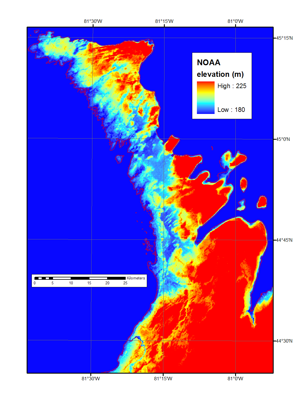
This is the ASTER 1" DEM. DEMs were made from the NIR stereo pairs of all ASTER images, and the lowest value was selected for each pixel.

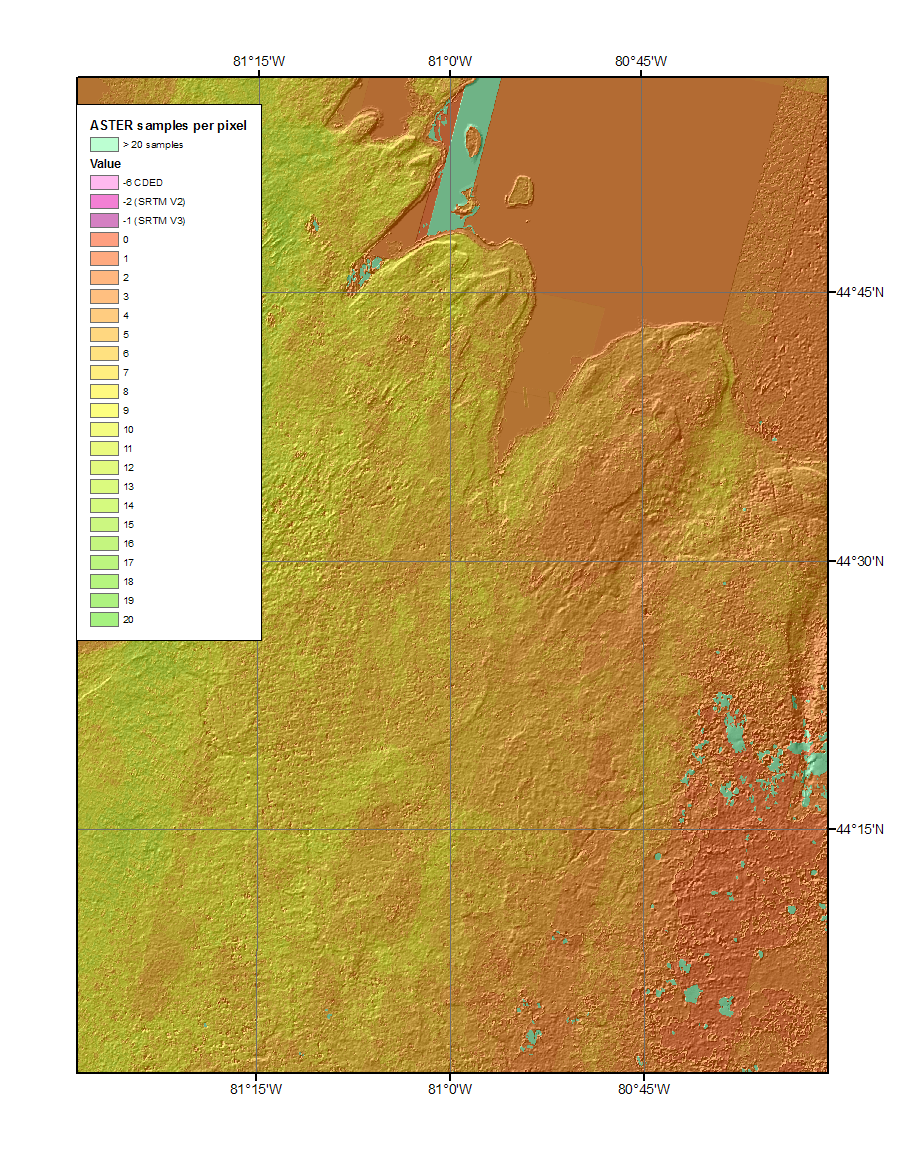
This shows the number of component images that built each pixel in the DEM above.

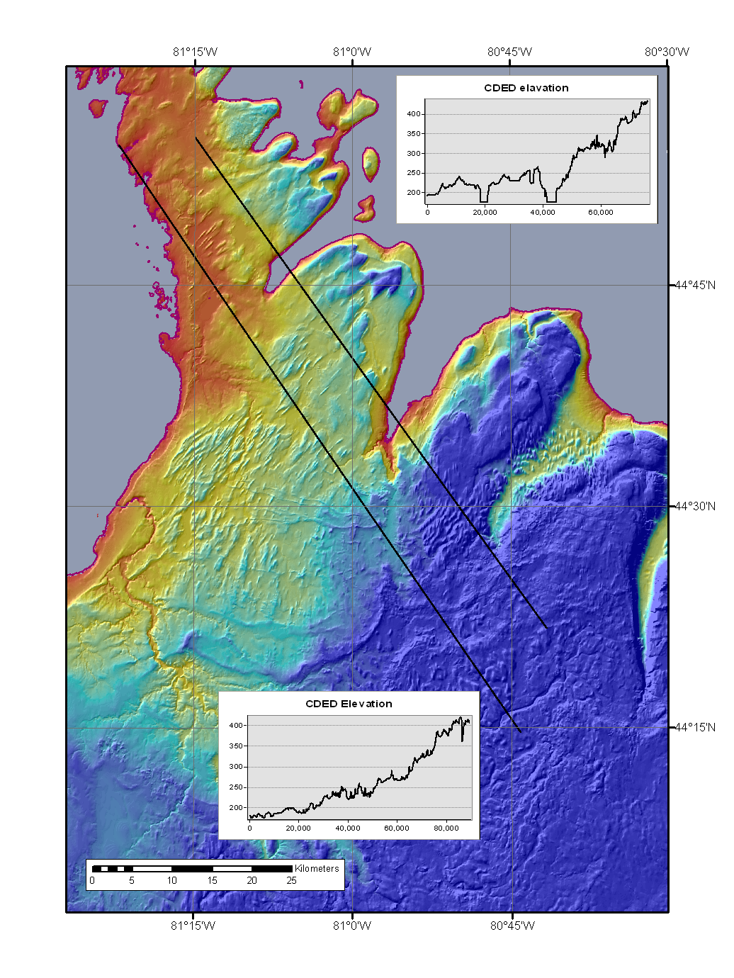
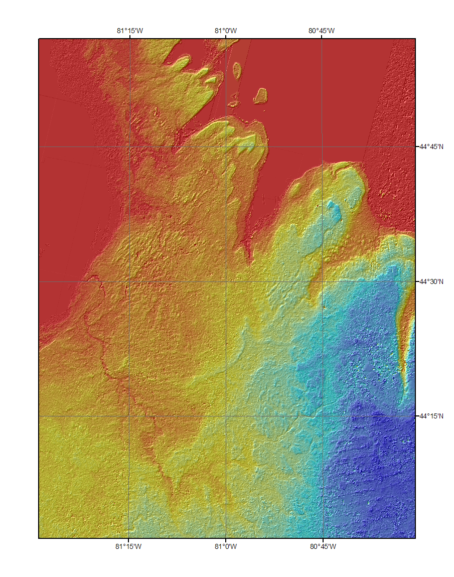
And this is the Canadian DEM. I like it better.

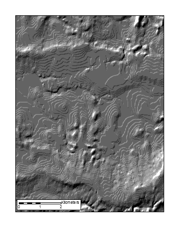
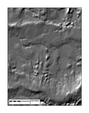
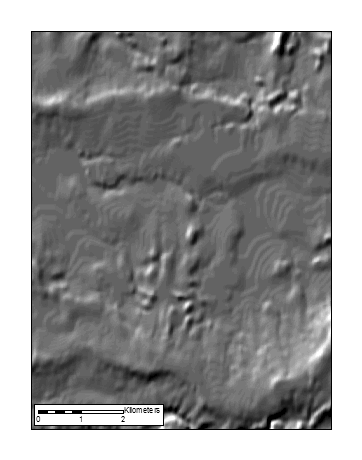
This is a detail of a simple shaded relief image of our CDED data. The one-meter increments of elevation look like the edges of rice paddies. (You would encounter similar problems with any DEM if you created a shaded relief image at a finer resolution than the DEM.)	This image is made from a smoothed (3-cell radius) version of the DEM. The model generally yields a one-byte image with values from 0 to 255. ArcMap gives you extensive control over raster display, but it defaults to a stretch between (mean-2*stddev) and (mean+2*stdev). As the standard deviation of shaded smooth DEM is smaller, the contrast gets kicked up.	This is the same as the second image, but a customized min-max stretch was used to match the stretch of the first image

If the size of a data cell is smaller than a screen pixel, information can fall through the cracks. If a shaded relief image is highly textured at sub-pixel resolution, the particular cell that is sampled for pixel display is essentially random, and the landscape is poorly portrayed. Bilinear pyramids can solve this problem. Some software, such as ArcMap, creates a hierarchy of lower resolution images for every raster data set that it displays. This allows it to throw a large image up on the screen very quickly when you are zoomed out. By default, the lower resolution images are created by nearest-neighbor resampling of the higher-resolution data. This does not help with the texture problem. However, you can right-click on a raster in ArcCatalog and ask to rebuild pyramids. When the rectangular pyramid window comes up, click the Environments button, open the Raster Storage section, and change the method from nearest neighbor to bilinear. This will fix the problem.

This does not solve all your problems. You may see how hills are beautifully dissected (Note: My mother would have wanted be to remind you that dissect does not rhymed with bisect.) by drainage patterns, but the hills themselves are not clearly defined. If you smooth a DEM you can create a shaded-relief representation of large features, but this is not so interesting. If you average the original DEM and the smoothed one, you can create a shaded-relief image that shows everything. You can fiddle with smoothings (and maybe multiple smoothings) and weights to optimize the image. Don't forget to preserve flat water bodies and to make bilinear pyramids.

As a landscape is smoothed, the histogram of shade values will be compressed. Some software (.e.g. ArcMap) will stretch the histograms by default, but will give options to show raw images or whatever you want. Do what makes your landscape look good, but be careful if you are making image tiles that you want to edgematch.

Here are examples illustrating resolution bumping. All of them are shown with ArcMap's default contrast stretch.

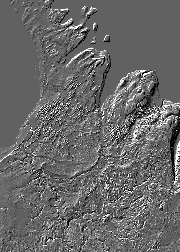
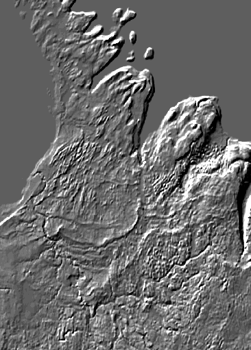
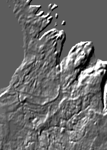
The first image is the same as the underlying layer in the second large image above, as repeated in detail in the second of the small images above. The DEM was smoothed, and the shaded-relief model that you see was made from that.	The second image image shows smoothing over a radius of 15 cells. (A purist could argue for the use of an elliptical smoothing window to compensate for latitude distortion. This is possible, but tedious. Resampling the DEM to an equidistant projection before processing would introduce a new set of artifacts.)	The third image shows smoothing over a radius of 36 cells. Large landforms are even more apparent.

Resolution bumping involves averaging two or more DEMs. Large landforms are visible from a distance, but fine detail is not lost. I chose a mix of 60% minimally (just enough to deemphasize stair-stepping), 20% smoothed to a 15-cell radius, and 20% smoothed to a 36-cell radius.

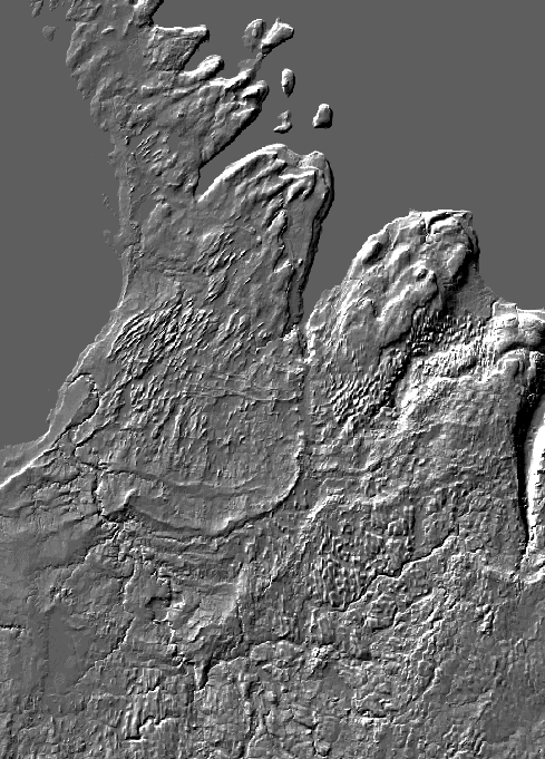
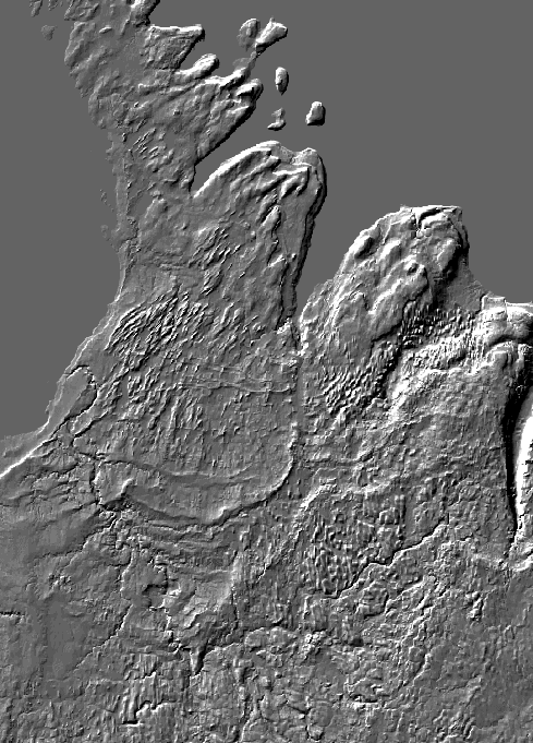
The first image is a weighted average of the shaded-relief images.	The second image is a shaded-relief model of a weighted average of the three versions of the DEM. This gives us a better range (I cannot explain why.), and also reduces artifacts by creating non-integer elevations.