Manuscript received October 31, 1997. This work was a collaborative effort of the U.S. and Japanese EOS/ASTER instrument teams, sponsored by the NASA EOS Project and ERSDAC.
A. Gillespie and J.S. Cothern are with the Department of Geological Sciences, University of Washington, Seattle, Washington 98195-1310, USA.
S. Rokugawa is with The University of Tokyo, Faculty of Engineering, 7-3-1 Hongo, Bunkyo-ku, Tokyo 113, JAPAN.
T. Matsunaga is with the Geological Survey of Japan, 1-1-3 Higashi, Tsukuba, Ibaraki 305, JAPAN.
S. Hook and A. Kahle are with the Jet Propulsion Laboratory 183-501, Pasadena, California 91109, USA
IEEE Log Number XXXXXXX
L and surface temperatures are important in global-change studies, in estimating radiation budgets and heat-balance studies, and as control for climate models. Emissivities are strongly indicative, even diagnostic, of composition, especially for the silicate minerals that make up much of the land surface. Surface emissivities are thus important for studies of soil development and erosion and for estimating amounts and changes in sparse vegetative cover for which the substrate is visible.
A new algorithm for determining land-surface temperatures (T) and emissivity (e) spectra for multispectral thermal infrared (8-12 çm) images has been developed for use with data from the Advanced Spaceborne Thermal Emission and Reflection Radiometer (ASTER), to be launched in June 1998 on the first of NASAs Earth Observing System polar-orbiting spacecraft, EOS-AM1. This temperature and emissivity separation (TES) algorithm relies on an empirical relationship between spectral contrast and minimum emissivity, determined from laboratory and field emissivity spectra, in order to equalize the number of unknowns and measurements so that the set of Planck equations for the measured thermal radiances can be inverted. TES is adaptable to multispectral images from imaging systems other than ASTER.
The key goals of TES are 1) to estimate accurate and precise surface temperatures especially over vegetation, water and snow, and 2) to recover accurate and precise emissivities for mineral substrates. The TES algorithm is designed to produce "seamless" images -- in other words, there should be no artifactual discontinuities, such as can be introduced by classification. TES embodies the simplest approach feasible consistent with the above goals. T (1 band) and e (5 bands) images will be available as standard products from EOS.
Thermal radiances vary with both T and e, which therefore must be recovered from the measurements. Surface temperatures are independent of wavelength and can be recovered from even a single band of radiance data, provided atmospheric characteristics can be specified and the surface emissivity is known. Except for water, vegetation and snow or ice, however, the emissivity of the land surface is not known a priori, but must be determined along with the temperature. The inversion for T and e is therefore under-determined: there is always at least one more unknown than the number of measurements. Separation of T and e data from the measured radiances therefore requires additional information, determined independently. In the TES algorithm, the additional data comes from the regression of minimum emissivity to spectral contrast of laboratory spectra. At least three or four spectral bands are required to measure the contrast in images. Therefore, it is necessary to make multispectral measurements in order to determine land surface temperatures. This is not the case for sea-surface temperature estimation, for example, because the emissivity spectrum of water is well known a priori.
The minimum number of bands necessary to recover land surface temperatures may be too small for surface composition mapping: because emissivity spectra of geologic materials can be quite complex, many emissivity studies require as many spectral bands in the 8-14 mm TIR window as possible. Current engineering limitations prevent TIR imaging spectroscopy from satellite, and multispectral sensors with a handful of spectral bands are a compromise.
This paper presents the TES algorithm, results of a validation experiment, and TES T and e images calculated from six-channel airborne TIMS images [1] processed to simulate ASTER data. Discussion focuses on the theoretically predicted and experimentally determined precision and accuracy estimates, and on the fundamental factors limiting TES performance.
ASTER has three bands in the visible and near-infrared (VNIR) spectral range (0.5-0.9 çm) with 15-m spatial resolution, six in the shortwave-infrared (SWIR: 1.6-2.4 çm) with 30-m resolution, and five in the thermal-infrared (TIR: 8-12 çm), with 90-m resolution [2,3]. These 14 bands are collected in three down-looking telescopes that may be slewed Ý8.5¯ (SWIR, TIR) or Ý24¯ (VNIR) in the cross-track direction. Combined with the FOV of Ý2.5¯, the maximum TIR view angle is thus 11¯. An additional backward-viewing telescope with a single band duplicating VNIR band 3 will provide the capability for same-orbit stereogrammetric data. The five TIR channels (ASTER bands 10-14) have spectral ranges of 8.125-8.475, 8.475-8.825, 8.925-9.275, 10.25-10.95, and 10.95-11.65 çm, respectively. ASTER's estimated TIR radiometric accuracy at 300K is 1¯K; at 240K it is 3¯K. Radiometric precision (NEDT) at 300K is <0.3¯K [4].
The ASTER team located all five TIR bands within the 8-12 çm atmospheric window to maximize geologic information. Because no spectral bands are located at the edges of the window, where atmospheric water absorbs ground emittance, it is not possible to estimate atmospheric profiles and parameters directly from ASTER images. The ASTER instrument team does compensate all measurements for atmospheric transmissivity and path radiance, and reports values for downwelling sky irradiance, all determined independently [5], so it is possible calculate accurate values of T and e.
The ASTER instrument is being provided by the Japanese Government under the Ministry of International Trade and Industry (MITI). The ASTER project is implemented through the Earth Remote Sensing Data Analysis Center (ERSDAC) and the Japan Resources Observation System Organization (JAROS), nonprofit organizations under MITI. JAROS is responsible for the design and development of the ASTER instrument, which will be built by the Nippon Electric Company (NEC), the Mitsubishi Electric Corporation (MELCO), Fujitsu, and Hitachi.
A surface radiates energy in proportion to its temperature (T) and emissivity (e). On the earth, atmospheric opacity restricts radiance measured by spacecraft to spectral windows at wavelengths of 3-5 and 8-14 mm. ASTER bands 10-14 lie within the TIR window of 8-14 mm. The basic problem in estimating T and e is that the data are non-deterministic: there are more unknowns than measurements because there is an e for each image band, plus T and atmospheric parameters. This is the case even if the scene is isothermal and consists of a single material of uniform texture and topographic slope and aspect. Consequently, even if atmospheric parameters are measured independently, at least one additional degree of freedom must be constrained independent of ASTER. There are several ways to constrain the extra degrees of freedom, resulting in a variety of approaches and algorithms to T and e separation. Below, the important equations governing TIR remote sensing and previous solutions are reviewed. The TES algorithm is then introduced and its performance is evaluated.
Conceptual framework for TIR remote sensing
Temperature is not an intrinsic property of the surface; it varies with the irradiance history and meteorological conditions. Emissivity is an intrinsic property of the surface and is independent of irradiance. The radiance from a perfect emitter (i.e., a blackbody for which e = 1) is exponentially related to temperature, as described by Planck's Law. The radiance R from a real surface, however, is less by the factor e: Rl = el Bl, where B is the blackbody radiance and l is wavelength (çm). ASTER integrates radiance emitted from a number of surface elements. It is attenuated during passage through the atmosphere, which also emits TIR radiation. Some of this radiance is emitted directly into the scanner ("path radiance"); some strikes the ground and is then reflected into the scanner. For most terrestrial surfaces the reflectivity r and e are complements (Kirchhoff's Law): rl = 1 - el. A simplified expression for the measured radiance L is:
For most terrestrial surfaces ~0.7<e<1.0, although surfaces with e<0.85 are probably restricted to deserts [6]. Radiance emitted at 10 çm from a surface at 300 K is on the order of 10 W m-2 çm-1 sr-1. For a sea-level summer scene, typical order-of-magnitude values of the atmospheric variables estimated by the LOWTRAN7 atmospheric model [7] are t >> 60%, ![]() >> 1.5 and
>> 1.5 and ![]() >> 0.6 W m-2 çm-1 sr-1. One effect of
>> 0.6 W m-2 çm-1 sr-1. One effect of ![]() is to reduce the spectral contrast of the ground-emitted radiance, because of Kirchhoff's Law. It is necessary to compensate for atmospheric effects, including
is to reduce the spectral contrast of the ground-emitted radiance, because of Kirchhoff's Law. It is necessary to compensate for atmospheric effects, including ![]() , if T and el are to be recovered accurately. Incident radiance from adjacent scene elements (pixels) varies with terrain roughness but is typically less than
, if T and el are to be recovered accurately. Incident radiance from adjacent scene elements (pixels) varies with terrain roughness but is typically less than ![]() and is usually ignored. Therefore, the remote-sensing problem reduces to L£teB(T)+tr
and is usually ignored. Therefore, the remote-sensing problem reduces to L£teB(T)+tr![]() +
+![]() . Equation 1 ignores the effects of the atmospheric point-spread function, as does TES.
. Equation 1 ignores the effects of the atmospheric point-spread function, as does TES.
Equation 1 describes only the radiance at a single wavelength, and only radiance from homogeneous isothermal surfaces. In practice, the radiance is measured over a band of wavelengths; however, errors due to this integration are small . At the 90-m scale of ASTER TIR pixels, many terrestrial surfaces consist of multiple components having different emissivity spectra and temperatures. Strictly speaking, each component adds to the number of unknowns, while the number of measurements is unchanged. ASTER TIR measurements for such complex surfaces are not sufficient to estimate all the unknowns; instead, it is necessary to determine only an effective T and e spectrum for each pixel.
Previous approaches
Inversion of the TIR equations for T and e have been attempted using deterministic and non-deterministic approaches. The former are restricted to areas for which one or more of the unknowns is known. Historically the chief reason for TIR measurements has been to estimate temperatures. This task is deterministic for important scenes for which e is not in question: the ocean [8], snowfields and glaciers, and closed-canopy forests. However, deterministic solutions require that the atmospheric parameters in equation 1 be measured directly and the measured radiance corrected for them, and this is not always feasible. Most ocean-temperature studies have utilized data from the Advanced Very High Resolution Radiometer (AVHRR), which has two channels, at 10.3-11.3 çm and 11.5-12.5 çm, thereby "splitting" the TIR spectral window. Joint analysis of the two "split-window" channels can compensate for atmospheric effects while solving for T [9-11]. Split-window algorithms rely on empirical regression relating surface radiance measurements to water temperatures. A version of the split-window algorithm has been developed for EOS/MODIS images [12].
Several authors have examined extending the "split-window" technique to land surfaces [13-15]. They all conclude, however, that large errors arise there due to unknown emissivity differences. Over land, the unknown emissivities are a greater source of inaccuracy than atmospheric effects. Inaccuracy of only 0.01 in e causes errors in T exceeding those due to atmospheric correction [16]. In general, land emissivities can not be estimated this closely, and must be measured if accurate kinetic temperatures are to be recovered. As a result, the usefulness of split-window methods for land is limited and the non-deterministic nature of TIR remote sensing must be addressed head-on. Many geologic studies, however, have utilized enhancements such as decorrelation stretching that do not recover T and e [17, 18]. A spectral-unmixing approach has been used to separate a non-linear measure of T from e, but the separation is imperfect [19].
In all, we examined 14 inversion methods for the general land-surface problem in creating TES. These algorithms: determine spectral shape but not T; require multiple observations under different conditions; assume a value for one of the unknowns; assume a spectral shape; or assume a relationship between spectral contrast and e. All require independent atmospheric correction. The temperature-independent spectral indices (TISI) [20]; thermal log residuals and alpha residuals [21]; and spectral emissivity ratios recover spectral shape [22,23]. The day-night method [24] increases the number of unknowns by 1 but doubles the number of measurements, making the problem over-determined. In practice, however, this approach magnifies measurement "noise" and requires "pixel-perfect" registration between the two images. Other techniques have been based on an assumed value for a "model" emissivity at one wavelength [25], or an assumed maximum emissivity value (normalized emissivity method) [26, 27]. These approaches are unsatisfactory for ASTER because inaccuracies tend to be high (Ý3¯K) and because tilts are introduced into the e spectra. Finally, the "alpha-derived emissivity" (ADE) method utilized an empirical relationship between the standard deviation and mean emissivity to restore amplitude to the alpha-residual spectrum, thereby recovering T also [21, 28, 29]. The ADE method, however, relies on Wien's approximation to invert equation 1, thereby introducing slope errors into the e spectrum. The Mean-MMD method avoids Wien's approximation and uses a modified ADE empirical relationship based on the minimum-maximum emissivity difference (MMD)[30].
The instrument team for the Moderate Resolution Imaging Spectroradiometer (MODIS), an imager of lower spatial resolution but wider field of view than ASTER and also carried on EOS-AM1, is considering an approach in which emissivities are specified by classifying VNIR/SWIR data [31]. Although important scene types such as vegetation are readily identified in the VNIR and have well known e spectra, classification is ineffective for many geological materials. It also creates sharp boundaries in images of gradual transitions.
Numerical modeling suggests that, for most scenes, the TES algorithm can recover temperatures with an accuracy and precision of 1.0-1.5¯K, assuming accurate radiometric measurements. Emissivities can be recovered with an accuracy and precision of 0.010-0.015. TES's performance over land and sea are comparable. ASTER TES temperature recovery is less accurate than the MODIS split-window algorithm for sea surfaces because ASTER resolution is better by an order of magnitude and its SNR is accordingly lower. ASTER's data acquisition plan, however, is focused on the land surface. Major limitations on algorithm performance arise from two main sources: 1) the reliability of the empirical relationship between emissivity values and spectral contrast; and 2) compensation for atmospheric factors. Measurement accuracy and precision contribute to TES errors, but to a lesser degree. Accuracies and precisions are of the same size, but arise from different sources. Inaccuracies are due mainly to errors in atmospheric compensation, which are probably systematic; imprecision arises mainly from scatter in the emin-MMD regression.
Theoretical basis for the TES algorithm
Figures 2 and 3 are flow diagrams of the TES algorithm. Below, the steps of the TES algorithm are presented in sufficient detail to permit regeneration of the processing code. The input ASTER image data sets consist of "Land-Leaving TIR Radiance", L', and sky irradiance, ![]() , together comprising an ASTER standard product (AST09) [5]. These calibrated data have been compensated for ASTER filter transmissivities and other instrument effects. Several TES parameters may be adjusted from their default values as the need arises. These parameters are identified in Figure 1 and below. The output data sets consist of the five emissivity images (AST05), corresponding to ASTER channels 10-14, and a single image of surface temperature, T (AST08).
, together comprising an ASTER standard product (AST09) [5]. These calibrated data have been compensated for ASTER filter transmissivities and other instrument effects. Several TES parameters may be adjusted from their default values as the need arises. These parameters are identified in Figure 1 and below. The output data sets consist of the five emissivity images (AST05), corresponding to ASTER channels 10-14, and a single image of surface temperature, T (AST08).
Estimating the surface temperature and subtracting reflected sky irradiance (NEM module)
The kinetic or "thermodynamic" temperature is estimated using the normalized emissivity approach. Essentially, emax is assumed in order to calculate a temperature and the other emissivities. A value of 0.99, characteristic of vegetation and water, is assumed to start with. If the NEM estimates of e have low contrast, it is likely that the initial assumption was nearly correct, and an empirically based process, described below, is used to refine emax. If the contrast is high, the surface is probably rock or soil, and a lower value of emax = 0.96, characteristic of those materials, is assumed and processing is restarted. For rock and soil, this lower default value cannot be refined. For all materials in the ASTER spectral library, emax is 0.94-1.00. Therefore, the estimated kinetic temperatures should be within Ý3¯K at 340 K, and within Ý2¯K at 273 K.
Upon entry to the NEM module, radiance R is estimated by R'=L'-(1- emax)![]() . The NEM temperature is taken to be the maximum temperature Tb estimated from the radiances Rb for the different image channels b (b=10-14 for ASTER):
. The NEM temperature is taken to be the maximum temperature Tb estimated from the radiances Rb for the different image channels b (b=10-14 for ASTER):
 (2)
(2)
For samples with low contrast, emax may be refined to improve accuracy. For near-graybodies, measurement error is the dominant source of spectral variance: the best value for emax minimizes the variance n of the NEM emissivities. Plotting n against emax yields an upwards-opening parabola. A new value of emax may be found by calculating ![]() for emax=0.92, 0.95 and 0.97, in addition to 0.99, and fitting a parabola to the data. If this curve has a minimum for 0.9< emax< 1.00, it indicates the best estimate of emax. In this case, the NEM module is executed again to find new NEM emissivities.
for emax=0.92, 0.95 and 0.97, in addition to 0.99, and fitting a parabola to the data. If this curve has a minimum for 0.9< emax< 1.00, it indicates the best estimate of emax. In this case, the NEM module is executed again to find new NEM emissivities.
Ratio algorithm (RATIO module)
The relative emissivities, bb, are found by ratioing the NEM emissivities, calculated from the NEM T and the atmospherically corrected radiances, to the average emissivity:
Because emissivities themselves are generally restricted to 0.7 <eb < 1.0, 0.75 < bb < 1.32. The errors in b due to inaccuracy in the NEM T are systematic but less than the random errors due to NEDT, for 240 < T < 340 K. Warping of the b spectrum is below the threshold of detectability for ASTER data.
Estimating TES emissivities and temperature (MMD module)
The b spectrum must next be scaled to actual emissivity values, and the surface temperature must be recalculated from these new emissivities and from the atmospherically corrected radiances. These TES T and e values comprise the ASTER Standard Products. An empirical relationship predicting emin from MMD is used to convert bb to eb. We established this regression using laboratory reflectance and field emissivity spectra [34], as discussed below.
The first step in the MMD module is to find the spectral contrast:
where MMD' is the corrected contrast, NEDe=0.0032 is calculated from NEDT=0.3¯K at 300K, and the coefficient c was determined empirically. Equation 6 improves the accuracy of TES for graybodies, but at the expense of precision. We have found that if MMD<0.03, the loss of precision becomes unacceptable. Therefore, when this is the case, MMD is not calculated and emin is not found from equation 5 but instead is set to 0.983, a value appropriate for graybodies such as vegetation, and processing continues.
The NEM T is likely to be in error by up to 3¯K because the assumed value of emax may be inaccurate. This inaccuracy can be reduced by calculating a TES T from the measured, atmospherically corrected radiances R and the TES emissivity spectrum:
where b* is the ASTER band for which emissivity eb is maximum (and correction for ![]() is minimum).
is minimum).
Final correction for sky irradiance and bias in bThe TES e values are more accurate than the NEM values used to estimate reflected ![]() . Recalculation of reflected
. Recalculation of reflected ![]() based on the TES e spectrum improves accuracy further. The TES e values are used to make a final single (non-iterative) correction to L' , and then new estimates of NEM e are calculated and then used to recalculate the b spectrum (Eq. 3). The improved TES e and T are then calculated as before. For a variety of simulated and real radiance measurements, the "refined" TES emissivities changed by as much as 0.01; therefore, this final correction is worth doing. Experience shows that there is little gain with iteration.
based on the TES e spectrum improves accuracy further. The TES e values are used to make a final single (non-iterative) correction to L' , and then new estimates of NEM e are calculated and then used to recalculate the b spectrum (Eq. 3). The improved TES e and T are then calculated as before. For a variety of simulated and real radiance measurements, the "refined" TES emissivities changed by as much as 0.01; therefore, this final correction is worth doing. Experience shows that there is little gain with iteration.
Quality assurance
The TES algorithm applied to ASTER data will report on its performance and on the accuracy and precision of its T and e products. The report will take the form of a header record and a 3-byte data plane. The QA data will include flags to report on the optional paths through TES, described above. Of central interest is the reported reliability of the TES T and e data. This is assessed by numerical simulation and by algorithm execution on different images simulated from laboratory and field spectrometer data [34]. TES performance depends strongly on the ratio of ![]() to L', and on MMD, indicators that can be assessed pixel-by-pixel during operation. It is anticipated that this information, together with the results of the numerical simulations, will be used to generate the QA data. Additionally, TES performance is affected by the proximity of clouds. This information will be reported in the QA plane and incorporated in the performance assessment.
to L', and on MMD, indicators that can be assessed pixel-by-pixel during operation. It is anticipated that this information, together with the results of the numerical simulations, will be used to generate the QA data. Additionally, TES performance is affected by the proximity of clouds. This information will be reported in the QA plane and incorporated in the performance assessment.
Regression of emin onto MMD
The relationship between emissivity and spectral contrast was established by analysis of laboratory reflectance spectra, equivalent to emissivity by Kirchhoff's Law. The data were converted to ASTER pseudo-spectra and emin was found for each sample. Radiances were estimated, scaling emissivities by blackbody radiances calculated for T=300 K, and b spectra and its MMD were calculated. The emin data were then regressed to the MMD values. They are related by a simple power law (Fig. 4; eq. 5). The regression parameters are insensitive to temperature. Although the regression parameters are defined empirically, the relationship itself is reasonable and physically predictable if deviation from blackbody behavior is due to molecular resonance localized in narrow reststrahlen features. The regression chosen for the TES algorithm uses emin rather than mean emissivity as in the Mean-MMD algorithm, because it improved the correlation. The MMD was used because, for most spectra, it was just as good and faster to calculate than other measures of spectral complexity, such as variance.
The critical assumption that this regression applies to the entire gamut of surface materials has been tested and appears to be valid. A different set of 31 reflectance spectra (35, 36) yielded nearly identical regression coefficients (H. Tonooka, Ibaraki Univ., Japan, pers. comm., 1996), as did field emissivity spectra of Australian rocks (n=91) collected using the Jet Propulsion Laboratory's çFTIR spectrometer (34). Hundreds of airborne MIRACO2LAS CO2 laser reflectance spectra, with a narrower window than the five ASTER TIR bands, yielded a regression having similar overall characteristics (T. Cudahy, CSIRO, pers. comm., 1996).
Performance in the presence of uncompensated atmospheric effects
If atmospheric correction is inaccurate, the residual effects can degrade the performance of TES. ASTER band 10 is more affected by atmospheric absorption and emission than the other ASTER bands, because it is located closest to the edge of the TIR atmospheric window. Numerical simulation suggests that, under these conditions, TES performance may be improved by eliminating ASTER band 10, and running TES on ASTER bands 11-14. This necessitates using a different emin - MMD regression, and different test values and constants throughout the algorithm. These alternative regressions have been calculated and are included in the TES code, but are not reported here. Once the TES T has been found from the subset of bands, it is used to calculate the emissivity spectrum for all five bands.
Numerical simulation results
Overall, the TES algorithm operating on error-free input radiances can recover temperatures for a wide range of surfaces within 1.5¯K and emissivities within 0.015. For numerically simulated radiance emitted from surfaces at 300K, based on the field emissivity spectra in our library, 95% of the recovered temperatures were within 1.5¯K and 68% (1 std. deviation) were within 0.3¯K, for example. TES performance is not related to scene composition in general, but to the scatter about the emin-MMD regression line, scatter which is largely independent of MMD (Fig. 4). Monte Carlo simulation shows that the scatter of recovered temperatures due to measurement error is about the same as that due to the inherent scatter about this regression line. Recovered emissivities show little bias, but err systematically by an amount proportional to the error in temperature: if TES overestimates T by 1¯K at 300 K, it will tend to underestimate e by ~0.017. Numerical simulation results are discussed at length by Gillespie et al. [33].
Tests on simulated ASTER images
Three ASTER images (Fig. 5) were simulated from calibrated TIMS overflights of Castaic Lake and Lake Tahoe, both in California, and of the south coast of Hawaii [39]. These images are used to test T and e recovery over water targets (low MMD). Three additional images have been prepared over a single geologic target, the playa in Railroad Valley, Nevada, and test recovery over land areas having high MMD (Figs. 6, 7). TIMS has similar NEDT and spectral bands to ASTER. Radiosonde atmospheric probes and Reagan Sun Photometer measurements of total water vapor, together with LOWTRAN 7 and MODTRAN2 atmospheric models [7, 37], were used to estimate t, ![]() and
and ![]() at the time of overflight [38]. Surface radiant temperatures were measured with calibrated Everest radiometers; water temperatures were measured with buoys.
at the time of overflight [38]. Surface radiant temperatures were measured with calibrated Everest radiometers; water temperatures were measured with buoys.
The Castaic Lake image (Fig. 5a) is of a reservoir, the earthen dam that impounds it, and sparsely vegetated hills [38]. Lake surface temperatures were 287.9 Ý0.3 K (n=49). TIMS radiances, with correct emissivities specified, indicate a water temperature of 289.0Ý1.6 K, suggesting from inaccurate atmospheric compensation. TES T was ~290.6 K, and the average emissivities were correspondingly low (~0.05). We attribute the inaccurate atmospheric to incorrectly calibrated hygristors in the radiosondes, a problem that was corrected in 1997.
The Lake Tahoe image includes the lake and forested, snowy mountains in addition to Dollar Point, a subdivision shown in Figure 5b. Field measurements of water, air and melting snow temperatures were ~280.3, ~283.1 and ~273.1 K, respectively. TES T values of water, forest and snow were 281.0Ý0.4, 283.9Ý0.6 and 273.7Ý0.4 K, respectively. Assuming forest and air temperatures were the same, the mean TES T's were systematically 0.4-0.8¯K too high, but within the uncertainty predicted from the numerical simulation studies. TES e spectra for Lake Tahoe were consistent with Lake Castaic.
The Hawai'i image shows an active lava flow entering the ocean near Kapa'ehu, accounting for the plume-like patterns in the water and for the wide range of temperatures there. A cloud of steam drifts west (left) from the entry point. Radiometric ocean temperatures measured three days before overflight were ~296 K, rising to ~330 K near the lava [38]. TES T ocean temperatures were 305Ý0.6 K, ~9 ¯K higher than the earlier radiometric temperatures. Emissivities recovered for the ocean were too low by 0.05-0.02 (bands 10 and 12, respectively). Uncorrected absorption and emission by SO2 and other gases from the lava may account for some of the discrepancies.
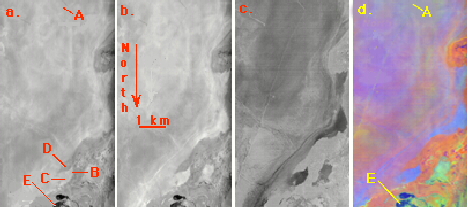
Railroad Valley images for three successive years (1995-1997) were analyzed. Figure 6 shows the playa, shallow ponds surrounded with reeds, and alluvial fans in 1996. Figures 6a, 6b and 6c show radiance, TES T, and TES e images, respectively; Figure 6d is a decorrelation-stretched false-color version of the same scene, indicating clearly the spectral homogeneity of the playa validation site (A). Results from 1995-96 were consistent with those from California and Hawaii. Running TES without band 10 cut pond temperature discrepancies in half. After correcting the radiosondehygristor calibration in 1997, TES emissivities for the pond and playa sites were brought into agreement with and laboratory and field measurements (Fig. 7). Precisions for e for homogeneous areas on the images were <0.006. We attribute some of the rms "error" of 0.018 for the playa to difficulties in comparing spectra made at different scales (6.4 m vs. 10 cm). TES pond temperatures were 290.8Ý0.4 K, 1.7¯K less than the buoy temperatures. Because of evaporation, water skin temperatures may be as much as 4¯K lower than buoy temperatures. TES temperatures of 314.2 Ý0.3 K for playa site E were indistinguishable from Everest radiant temperatures of 314.3Ý0.9 K (n=99, e=0.93).
Correcting for sky irradiance in the TES algorithm reduced apparent water temperatures by ~0.2 ¯K for the California and Nevada sites, and ~0.5 ¯K for Hawaii.
TES is sensitive to errors in spectral contrast because emissivity amplitude and hence temperature depend on MMD. Therefore, incomplete removal of atmospheric effects in even a single channel may reduce accuracies of the recovered T and e significantly.
Scatter about the emin-MMD regression line appears to be a property of natural surfaces, and not experimental artifact. It is a fundamental feature of TES that limits its performance. For high-MMD scenes the scatter is coincidentally equivalent to the ASTER NEDT of ~0.3 ¯K, and to engineering predictions of ~1¯K radiometric. The MMD effects are most serious for graybodies, such as vegetation and water. For these important scene types random measurement errors affecting MMD can be amplified in the final T and e products.
Improvements in ASTER sensitivity and noise levels would translate into improved TES precision over natural graybodies. However, even for NEDT=0, TES could not match the accuracy of dedicated sea-surface temperature algorithms, because these presume that e is known and TES does not. For geologic surfaces, the inherent variability on the emin-MMD plane, not the NEDT, is the major source of uncertainty.
Atmospheric compensation may be the effective limit on TES performance with ASTER data during the EOS mission. For most scenes, the critical parameters are atmospheric transmissivity and path radiance. Errors in correction for these parameters propagate directly into T and e. For many scenes, sky irradiance reflected from the scene is of minor significance: for example, at Castaic Lake it accounted for only 0.2 ¯K. For humid atmospheres or warm atmospheres over cold scenes, however, the correction for reflected sky irradiance may be larger, even the most important factor limiting TES performance.
Most soil or rock surfaces, and open-canopy vegetation, contain multiple components at the 90-m scale of ASTER pixels. Therefore, performance of TES for mixed pixels is of interest. Mixtures of scene materials fall near the emin-MMD regression line if the endmembers do also. Potential sources of error include admixture of blackbody cavity radiation from rough surfaces, since ideal blackbodies fall above the regression line. Theoretical studies with radiosity models suggest that these effects will be minor because multiple-scattering contributions rarely exceed ~20% of the total radiance from natural surfaces.
It may be useful to apply TES to multispectral TIR images from a variety of imaging systems. To be effective, TES probably requires at least three or four bands of data: numerical simulations show that uncertainties become larger as the number of bands is reduced further. It is possible for TES to run, for example, on only four of the five bands acquired by ASTER with little degradation in performance, whereas for two bands the products are only half as precise. As the number of bands is increased beyond ten or twelve, the emin-MMD regression increasingly limits performance compared to other algorithms. For imaging spectroscopy studies, it is likely that a different temperature/emissivity separation algorithm will be devised. Extension to wide-angle scanners may require compensation for directional effects at high scan angles such as predicted in MODIS data (Ý45¯) that have not been considered in writing TES.
TES requires further testing on calibrated, atmospherically corrected TIR data before routine use by the remote-sensing community. However, we conclude that TES is a useful and general algorithm for recovering land surface temperature and emissivities from multispectral TIR imaging systems. The fundamental limitations are the variability in the emin-MMD relationship for natural surfaces, and atmospheric characterization and correction. Future refinements of TES may be possible, but performance characteristics reported in this discussion are probably close to the ultimate limits achievable with its approach.